Abstruct Data Type¶

Array & Linked list¶

Array¶

Data are stored continuously in memory.
Often fixed size. (but not for dynamic array)

Operation	Time
insert	$O(n)$
remove	$O(n)$
access	$\blue{O(1)}$
find	$O(n)$

Linked List¶

Each data is stored in a node scattered in memory.
Can be easily extended.
Use more space to store pointers to next.

Singly Linked List¶

C++

class Node {
private:
  int val;
  Node *next;
public:
  Node(int = 0, Node* = nullptr);

  int retrieve() const;
  Node *next() const;

  void push_front();
  int pop_front();
}

Operation	Time
insert	$\blue{O(1)}$
remove	$\blue{O(1)}$
access	$O(n)$
find	$O(n)$

Doubly Linked List¶

C++

class Node {
private:
  int val;
  Node *previous;
  Node *next;
public:
  Node(int = 0, Node* = nullptr);

  int retrieve() const;
  Node *next() const;

  void push_front();
  int pop_front();
}

Circular Linked List¶

The last node stores the pointer to the head node.

Stack & Queue¶

Stack¶

Reverse-Polish Notation

No ambiguity and no brackets are required.

Realized by stack.

The stack can be implemented using either an array or a linked list (std::deque in C++)

Follows the principle of Last-In-First-OUT.
push() to add element to the top of stack & pop() to remove the top element.
ALL implemented in $O(1)$.

C++

class ArrayStack {
private:
  std::vector<int> stack;

public:
  int size() const;
  bool empty() const;

  void push(int val) {
    stack.push_back(val);
  }
  int pop() {
    int num = top();
    stack.pop_back();
    return num;
  }
  int top();
};

C++

class LinkedListStack {
private:
  Node *top;
  int size;
public:
  int size() const;
  bool empty() const;

  void push(int val) {
    Node *node = new Node(val);
    node->next = top;
    top = node;
    size++;
  }
  int pop() {
    int num = top();
    Node *tmp = top;
    top = top->next;
    delete tmp;
    size--;
    return num;
  }
  int top();
};

Operation	Time
`push()`	$\blue{O(1)}$
`pop()`	$\blue{O(1)}$
`peek()`	$\blue{O(1)}$

Queue¶

Follows the principle of First-In-First-OUT.
push() to add element to the front of queue & pop() to remove the last element.

C++

class ArrayQueue {
private:
  int *val;
  int front;
  int size;
  int capacity;
public:
  ArrayQueue(int cap) {
    val = new int[cap];
    capacity = cap;
    front = 0;
    size = 0;
  }

  ~ArrayQueue() {
    delete[] val;
  }

  int capacity();
  int size();
  bool empty;

  void push(int num) {
    if (size == capacity) return;
    int rear = (front + size) % capacity;
    val[rear] = num;
    size++;
  }
  int pop() {
    int num = front();
    front = (front + 1) % capacity;
    size--;
    return num;
  }
  int front();
};

Implemented by circular array.

C++

class LinkedListQueue {
private:
  Node *front, *rear;
  int size;
public:
  LinkedListQueue() {
    front = nullptr;
    rear = nullptr;
    size = 0;
  }

  ~LinkedListQueue();

  int size();
  bool empty();

  void push(int val) {
    Node *node = new Node(val);
    if (front == nullptr) {
      front = node;
      rear = node;
    } else {
      rear->next = node;
      rear = node;
    }
    size++;
  }
  int pop() {
    int num = front();
    Node *tmp = front;
    front = front->next;
    delete tmp;
    size--;
    return num;
  }
  int front();
};

Operation	Time
push()	$\blue{O(1)}$
pop()	$\blue{O(1)}$
peek()	$\blue{O(1)}$

Example: Maze Routing¶

BFS: use queue
DFS: use stack

Hash Table¶

Hash table is a higly efficient data structure.

Establishes a mapping between keys and values.
Load Factor: the average number of objects per bin. $$ \lambda = \frac{n}{M} $$
Probability of at least one collision $$ 1 - \frac{M(M-1)\cdots(M-n+1)}{M^n} $$

Operation	Array	Linked List	Hash Table
insert	$O(n)$	$\blue{O(1)}$	$\blue{O(1)}$
remove	$O(n)$	$\blue{O(1)}$	$\blue{O(1)}$
access	$\blue{O(1)}$	$O(n)$	$\blue{O(1)}$
find	$O(n)$	$O(n)$	$\blue{O(1)}$

Hash Collision¶

If the return of hashFunction(key) are the same, e.g.

Text Only

114514 % 100 = 14
145114 % 100 = 14

this situation is called hash collision.

Hash collision is inevitable because the input space is much larger than the output space.

We can reduce hash collisions by resizing the hash table, but we'd better improve the hash table data structure, since resizing a hash table is time-consuming and space-consuming.

Separate Chaining¶

Each bucket stores a linked list, containing all colliding elements.

Open Addressing¶

Linear Proding¶

If the bucket already contains an element, linearly traverse forward the conflict position to insert or search elements.

e.g. If index $n$ has already store a pair, we jump to $n+1$, if so, then $n+2$, $n+3$, etc.

Quadratic Proding¶

Similar to linear proding, if the bucket already contains an element, traverse by skipping a square of the number of prodes forward the conflict position to insert or search elements.

e.g. If index $n$ has already store a pair, we jump to $n+1$, if so, then $n+2$, $n+4$, etc.

Double Hashing¶

Uses two hash functions $h_1(k), h_2(k)$ for proding.

\[ h(k) = h_1(k) + i \cdot h_2(k) \]

Then Linear Proding can be shown as $h(k) = h_1(k) + i$, where $h_2(k) = 1$

Quadratic Proding can also be shown as $h(k) = h_1(k) + c_1 + c_2 \cdot i$, where $h_2(k) = c_1 + c_2 \cdot i$

Hash Algorithm¶

The methods given above can be used to solve hash collision. However, they cannot reduce the frequency of hash collisions. So we need to design some algorithms in order to avoid collisions.

Common Hash Algorithm¶

In practice, we usually use some standard hash algorithms, such as MD5, SHA-1, SHA-2, and SHA-3. They can map input data of any length to a fixed-length hash value.

Tree¶

All nodes will have zero or more child nodes or children
For all nodes other than the root node, there is one parent node
The degree of a node is defined as the number of its children.
- Nodes with degree zero are also called leaf nodes
For each node in a tree, there exists a unique path from the root node to that node
The height of a tree is defined as the maximum depth of any node within the tree
Ancestor of node $n$: any node $y$ on the (unique) path from root $r$ to node $n$ is an ancestor of node $n$
Descendent of node $n$: any node $y$ for which $n$ is an ancestor of $y$

A recursive definition of a tree

A degree-0 node is a tree
A node with degree $n$ is a tree if it has $n$ children and all of its children are disjoint trees (i.e. with no intersecting nodes)

Code

C++

// TreeNode structure definition
struct TreeNode {
  int value;
  std::vector<TreeNode*> children;

  TreeNode(int val) : value(val) {}
};

// Helper function to check if there are duplicate nodes (disjoint check)
bool areDisjoint(TreeNode* node, std::unordered_set<TreeNode*>& visited) {
  if (visited.count(node)) return false;  // Node already visited

  visited.insert(node);  // Mark this node as visited
  for (TreeNode* child : node->children) {
    if (!areDisjoint(child, visited)) {
      return false;  // If any child violates the disjoint rule
    }
  }
  return true;
}

// Main function to check if the tree is valid
bool IsTree(TreeNode* root) {
  if (root == nullptr) return true;  // Empty tree is valid

  std::unordered_set<TreeNode*> visited;  // To track visited nodes
  if (!areDisjoint(root, visited)) return false;  // Check disjoint condition

  // Verify the recursive tree structure
  for (TreeNode* child : root->children) {
    if (!IsTree(child)) return false;  // Recursively check all children
  }
  return true;
}

Operations¶

Access the root
Given an object in the container:
- Access the parent of the current object
- Find the degree of the current object
- Get a reference to a child
- Attach a new sub-tree to the current object
- Detach this tree from its parent

C++ Implementation¶

Tree Traversal¶

Breadth-First Traversal¶

Visit all nodes at a given depth before descending a level

Place the root node into a queue
While the queue is not empty:
- Pop the node at the front of the queue
- Push all of its children into the queue

The order in which the nodes come out of the queue will be in breadth-first order

Depth-First Traversal¶

Pre-ordering¶

Post-ordering¶

Monte Carlo Tree Search¶

A randomized and principled tree search method

Binary Tree¶

A binary tree is a restriction where each node has exactly two children.

A full binary tree is where each node is a full node, or a leaf node.

Perfect Binary Tree¶

A perfect binary tree of height $h$ is a binary tree where

All leaf nodes have the same depth $h$.
All other nodes are full.

Theorems¶

A perfect binary tree of height $h$ has $2^{h+1} - 1$ nodes.
The height is $\Theta(\ln n)$.
There are $2^h$ leaf nodes.
The average depth of a node is $\Theta(\ln n)$:

\[ \begin{aligned} \frac{\sum_{k=0}^{h}k 2^k}{2^{h+1} - 1} &= \frac{h2^{h+1} - 2^{h + 1} + 2}{2^{h+1} - 1} = \frac{h(2^{h+1} - 1) - (2^{h+1} - 1) + 1 + h}{2^{h+1} - 1}\\ &= h - 1 + \frac{h + 1}{2^{h+1} - 1} \approx h - 1 = \Theta(\ln n) \end{aligned} \]

Complete Binary Tree¶

Recursive definition: a binary tree with a single node is a complete binary tree of height $h = 0$ and a complete binary tree of height $h$ is a tree where either:

The left sub-tree is a complete tree of height $h – 1$ and the right sub-tree is a perfect tree of height $h – 2$, or
The left sub-tree is perfect tree with height $h – 1$ and the right sub-tree is complete tree with height $h – 1$

More commonly, a complete is perfect except the last level, and the leaves in the last level are implemented from left side to the right side.

Theorems¶

The height is $h = \left\lfloor \lg n\right\rfloor$

Left-Child Right-Sibling Binary Tree¶

Store a general tree as a binary tree.

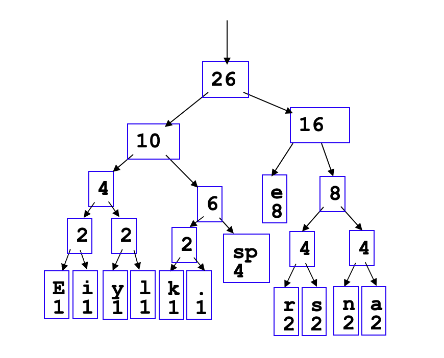
*Huffman Code¶

Reduce size of data.

Going left if a $0$
Going right is a $1$
Code word is only completed when a leaf node is reached.

Binary Search Tree¶

All objects in the left sub-tree to be less than the object stored in the root node.
All objects in the right sub-tree to be greater than the object in the root object.
The two sub-trees are themselves binary search trees.

Implementation¶

print()

In-order traversal
insert()
erase()

AVL Tree¶

A BST can easily degenerate into a linked list in some cases. In order to take advantage of BST properties, we need some operations to keep it balanced.

All operations are in $O(\log n)$

Cases¶

Case 1¶

Case 2¶

Case 3 (Only happen when erasing nodes)¶

Do the same as in Case 1 when erasing a node.

Heap¶

Binary Heap¶

A non-empty tree is a min-heap if

The key associated with the root is less than or equal to the keys associated with the sub-trees (if any)
The sub-trees (if any) are also min-heaps

Operation	Time
`push()`	$O(\log n)$
`pop()`	$O(\log n)$
`peek()`	$\blue{O(1)}$

Array Implementation¶

Start at index 1 when filling the array.

Given the entry at index k, it follows that:

The parent of node is a $k/2$
The children are at $2k$ and $2k + 1$

Fibonacci Heap¶

Consist of a group of trees satisfying the minimum-heap property.
The minimum key is always at the top of the trees.

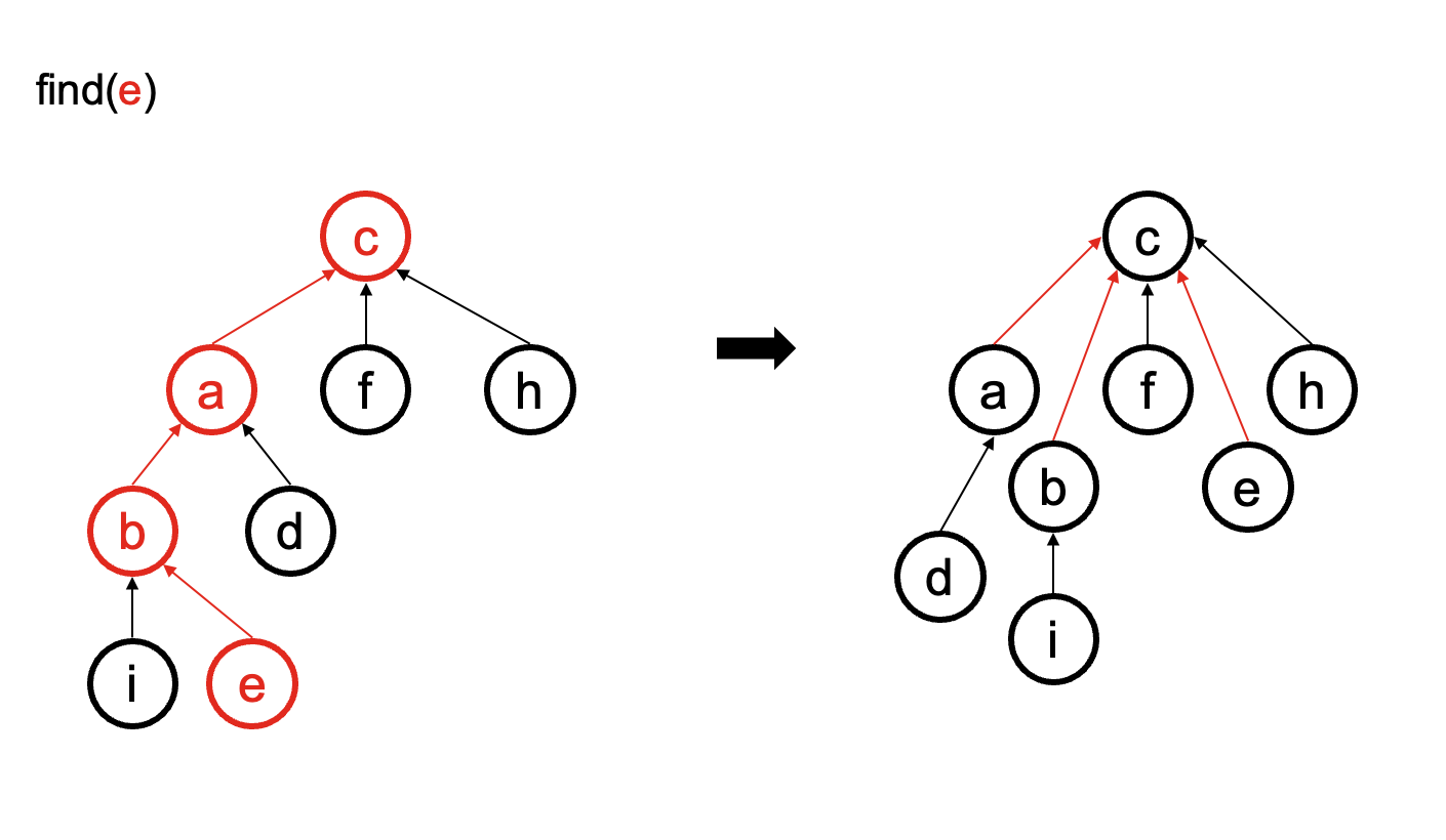
Disjoint Set¶

Worst case: $O(\log n)$ (or $O(n)$ without optimization)
Average case: $O(\alpha (n))$
Best case: $\Theta(1)$

About $\alpha (n)$

$\alpha(n)$ is the inverse of the function $A(i,j)$, that is

\[ \alpha (n) = \min \{i \mid A(i, i)\geq n\} \]

where $A(i,j)$ is the Ackermann function

\[ A(i,j) = \begin{cases} j+1, &i=0\\ A(i-1,1), &i>0, j=0\\ A(i-1, A(i, j-1)), &i>0, j>0 \end{cases} \]

Implementation¶

find(i)
- Find the root element of the tree that contains i.
set_union(i, j)
- Find the root elements of i and j.
- Update the parent of one root element to be the other root element.

Optimization 1: Union-by-rank¶

When two trees have the same height, the set specified first in the union will be the root of the merged set.

Point the root of the shorter tree to the root of the taller tree.
The height of the taller will increase if and only if the trees are equal in height.

Optimization 2: Path compression¶

The set specified first in the union will always be the root of the merged set.

C++

size_t Disjoint_set::find(size_t n) {
  if (parent[n] == n) {
    return n;
  } else {
    parent[n] = find(parent[n]);
    return parent[n];
  }
}

Operation	Array	Linked List	Hash Table
insert	\(O(n)\)	\(\blue{O(1)}\)	\(\blue{O(1)}\)
remove	\(O(n)\)	\(\blue{O(1)}\)	\(\blue{O(1)}\)
access	\(\blue{O(1)}\)	\(O(n)\)	\(\blue{O(1)}\)
find	\(O(n)\)	\(O(n)\)	\(\blue{O(1)}\)

Operation	Time
`push()`	\(O(\log n)\)
`pop()`	\(O(\log n)\)
`peek()`	\(\blue{O(1)}\)

Abstruct Data Type¶

Array & Linked list¶

Array¶

Linked List¶

Singly Linked List¶

Doubly Linked List¶

Circular Linked List¶

Stack & Queue¶

Stack¶

Queue¶

Example: Maze Routing¶

Hash Table¶

Hash Table¶

Hash Collision¶

Separate Chaining¶

Open Addressing¶

Linear Proding¶

Quadratic Proding¶

Double Hashing¶

Hash Algorithm¶

Common Hash Algorithm¶

Tree¶

Operations¶

C++ Implementation¶

Tree Traversal¶

Breadth-First Traversal¶

Depth-First Traversal¶

Pre-ordering¶

Post-ordering¶

Monte Carlo Tree Search¶

Binary Tree¶

Perfect Binary Tree¶

Theorems¶

Complete Binary Tree¶

Theorems¶

Left-Child Right-Sibling Binary Tree¶

*Huffman Code¶

Binary Search Tree¶

Implementation¶

AVL Tree¶

Cases¶

Case 1¶

Case 2¶

Case 3 (Only happen when erasing nodes)¶

Heap¶

Binary Heap¶

Array Implementation¶

Fibonacci Heap¶

Disjoint Set¶

Implementation¶

Optimization 1: Union-by-rank¶

Optimization 2: Path compression¶

评论